Calculus with Code

There is a lot of overlap between the fields of mathematics and programming, and there is computing software that implements mathematics with code, including MATLAB, Mathematica and SageMath.

While such programs are already capable of handling most mathematical tasks, including calculus of course, I'd still like to post some primitive code implementations (i.e. without using third-party modules like NumPy and considering floating-point errors) of the two major components of calculus, i.e. differentiation and integration, using Python, which I've learnt from my university programming methodology course, here. They also serve as demonstrations of the concept of higher-order functions, which they mathematically are as well.

Here, instead of deriving the symbolic expressions of the derivatives or integrals, the numerical methods of evaluating them are presented.

Differentiation

First Derivative

The following code snippet takes in a (real-valued) function f and returns a function that takes in a value a (on which f is differentiable) and returns the approximated first derivative of f, applying the first principle of differentiation.

$$f'(a) = \lim_{h \to 0}\frac{f(a+h)-f(a)}{h}=\lim_{x \to a}\frac{f(x)-f(a)}{x-a}$$

def derivative(f):
    h = 10 ** (-10) # hard-coded small value for accuracy
    return lambda a: (f(a+h) - f(a)) / h

Higher-order Derivatives

To compute the higher-order derivatives, one can use the following code snippet that involves self-composition of functions, or more formally: (positive) functional powers.

# Iterative functional composition implementation
def compose(f, pow):
    composed = lambda x: x # identity function
    for i in range(pow):
        composed = (lambda g: lambda x: f(g(x)))(composed)
    return composed

def higher_derivative(f, ord):
    return lambda x: compose(derivative(f), ord)(x)

degree_five_polynomial = lambda x: x ** 5 - x + 1
df, d5f = derivative(degree_five_polynomial), higher_derivative(degree_five_polynomial, 5)
print(df(0)) # -1.000000082740371, actual: -1
print(d5f(0)) # 0.0, actual: 0.0

Newton-Raphson Method

The Newton-Raphson method is an iterative algorithm that makes use of derivatives to approximate a root of a (real-valued) function $f$ (which is differentiable near the root), i.e. the value $a$ for which $f(a)=0$.

$$\text{Start from an initial guess } x_0,\; \text{ then for } n \geqslant 0:\; x_{n+1}=x_{n}-{\frac {f(x_{n})}{f'(x_{n})}}.$$

The following code implementation takes in a function f, an inital guess of the root value init, and optionally the number of decimal places d that the estimate should be accurate up to, then outputs the resulting approximated value.

def newtons_method(f, init, *d):
    if len(d) > 1:
        raise TypeError("Too many arguments")
    df = derivative(f) # reusing the derivative function above
    def improve(x):
        return x-(f(x)/df(x))
    tolerance = 10 ** (-15) # hard-coded small value for accuracy
    guess = init
    while abs(f(guess)) > tolerance:
        guess = improve(guess)
    return round(guess, d[0]) if d else guess

square = lambda x: x*x
sqrt_newton = lambda a: newtons_method(lambda t: square(t)-a, a/2)
print(sqrt_newton(2)) # 1.4142135623730951

Integration - Definite Integrals: Area under a Curve

note

Unless otherwise specified, the Riemann version of integrals is assumed to be default here.

The following code snippets approximate the area under the graph of a real function f between two given values a and b, applying the concept of Riemann sum) (rectangle rule).

$$\int _{a}^{b}f(x)\,dx\approx\sum _{i=1}^{n}f(x_{i}^{*})\,\Delta x_{i} \text{ where } x_0 = a,\; x_n = b,\; x_{i}^{*} \in [x_{i-1},x_i] \text{ and } \Delta x_i = \frac{b-a}{n}$$

The midpoint rule, trapezium rule, Simpson's rule and Boole's rule¹ are covered here.

Midpoint Rule

The midpoint rule approximates the definite integral by evauluating and summing over the values at the midpoints of a number of subintervals that partition the two given endpoints of the integral. It is 3rd-order accurate, i.e. it has an error of order $O(h^3)$.

$$\int_{a}^{b}f(x)dx \approx \Delta x\left[f\left(a+{\tfrac {\Delta x}{2}}\right)+f\left(a+{\tfrac {3\Delta x}{2}}\right)+\dots +f\left(b-{\tfrac {\Delta x}{2}}\right)\right]$$

An illustration of the midpoint rule in action (09glasgow09, CC BY-SA 3.0, via Wikimedia Commons).

The following code snippet makes use of the sum function that simulates the behaviour of summation.

def sum(term, a, next, b):
    result, curr_idx = 0, a
    while curr_idx <= b:
        result += term(curr_idx)
        curr_idx = next(curr_idx)
    return result

def integral_midpoint(f, a, b, dx):
    '''
    This function takes in the following parameters:-
    f: function to be integrated,
    a: lower limit of integration,
    b: upper limit of integration,
    dx: the length of each subinterval in the equal partition of the integration interval,
    and outputs the value of the integral approximated using the midpoint rule.
    '''
    add_dx = lambda x: x + dx
    return dx * sum(f, a+(dx/2), add_dx, b)

cube = lambda x: x*x*x
print(integral_midpoint(cube, 0, 1, 0.01)) # 0.24998750000000042, exact value: 0.25

Trapezium Rule

The trapezium rule is a technique that approximates the definite integral via linear functions passing through the endpoints of the subintervals, thereby resulting in trapeziums whose areas we can then sum over. It is 3rd-order accurate, i.e. it has an error of order $O(h^3)$.

$$\int _{a}^{b}f(x)\,dx \approx {\frac {h}{2}}{\Biggl (}f(x_{0})+2f(x_{1})+2f(x_{2})+2f(x_{3})+\dotsb +2f(x_{n-1})+f(x_{n}){\Biggr )} \text{ where } h=\frac{b-a}{n}$$

The sum function defined as above is reused in the following implementation.

A visualisation of the trapezium rule in action (Aravindh Vasu, CC BY-SA 4.0, via Wikimedia Commons)

def integral_trapezium(f, a, b, n):
    '''
    This function takes in the following parameters:-
    f: function to be integrated,
    a: lower limit of integration,
    b: upper limit of integration,
    n: number of subintervals in the partition of the integration interval,
    and outputs the value of the integral approximated using the trapezium rule.
    '''
    h = (b-a)/n
    def term(i):
        t, c = a + i * h, None
        if i == 0 or i == n:
            c = 1
        else:
            c = 2
        return c * f(t)
    return (h/2) * sum(term, 0, lambda i: i + 1, n)

cube = lambda x: x*x*x
print(integral_trapezium(cube, 0, 1, 50)) # 0.25010000000000004, exact value: 0.25 (set n = 50)

Simpson's Rule

The Simpson's rule is a refinement of the midpoint and trapezium rules in the sense that it has a better order of accuracy; it is 5th-order accurate, i.e. an error of order $O(h^5)$. This rule approximates the integral via a bunch of quadratic functions (parabolas).

The sum function defined as above is reused (again) in the following implementation.²

$$\int _{a}^{b}f(x)\,dx\approx \frac {h}{3}\left[f(a)+4f\left(a+h\right)+f(b)\right] \text{ where } h=\frac{b-a}{2}$$

def integral_simpson(f, a, b):
    '''
    This function takes in the following parameters:-
    f: function to be integrated,
    a: lower limit of integration,
    b: upper limit of integration,
    and outputs the value of the integral approximated using the Simpson rule.
    '''
    return integral_comp_simpson(f, a, b, 2) # check the "Composite Simpson's Rule" section for the definition of integral_comp_simpson

cube = lambda x: x*x*x
print(integral_simpson(cube, 0, 1)) # 0.25, exact value: 0.25

Composite Simpson's Rule

The composite Simpson's rule is a generalisation of the Simpson's rule that is useful in approximating the definite integral of a function over an interval on which it is not smooth.

One obtains the basic Simpson's rule by setting $n = 2$.

$$\int_{a}^{b}f(x)dx\approx{\frac {h}{3}}{\big [}f(x_{0})+4f(x_{1})+2f(x_{2})+4f(x_{3})+2f(x_{4})+\dots +2f(x_{n-2})+4f(x_{n-1})+f(x_{n}){\big ]} \text{ where } h=\frac{b-a}{n}$$

A visualisation of Simpson's rule in action (Aravindh Vasu, CC BY-SA 4.0, via Wikimedia Commons)

This was featured as a tutorial question of the aforementioned programming methodology course.

The following code implementation is my solution to the question, which also makes use of the sum function.

def integral_comp_simpson(f, a, b, n):
    '''
    This function takes in the following parameters:-
    f: function to be integrated,
    a: lower limit of integration,
    b: upper limit of integration,
    n: number of subintervals in the partition of the integration interval,
    and outputs the value of the integral approximated using the composite Simpson rule.
    '''
    h = (b - a)/n
    def term(i):
        t, c = a + i * h, None
        if i == 0 or i == n:
            c = 1
        elif i % 2 == 1:
            c = 4
        elif i % 2 == 0:
            c = 2
        return c * f(t)
    return (h/3) * sum(term, 0, lambda i: i + 1, n) # sum function defined as above

cube = lambda x: x*x*x
print(integral_comp_simpson(cube, 0, 1, 10)) # 0.25, exact value: 0.25 (set n = 10)

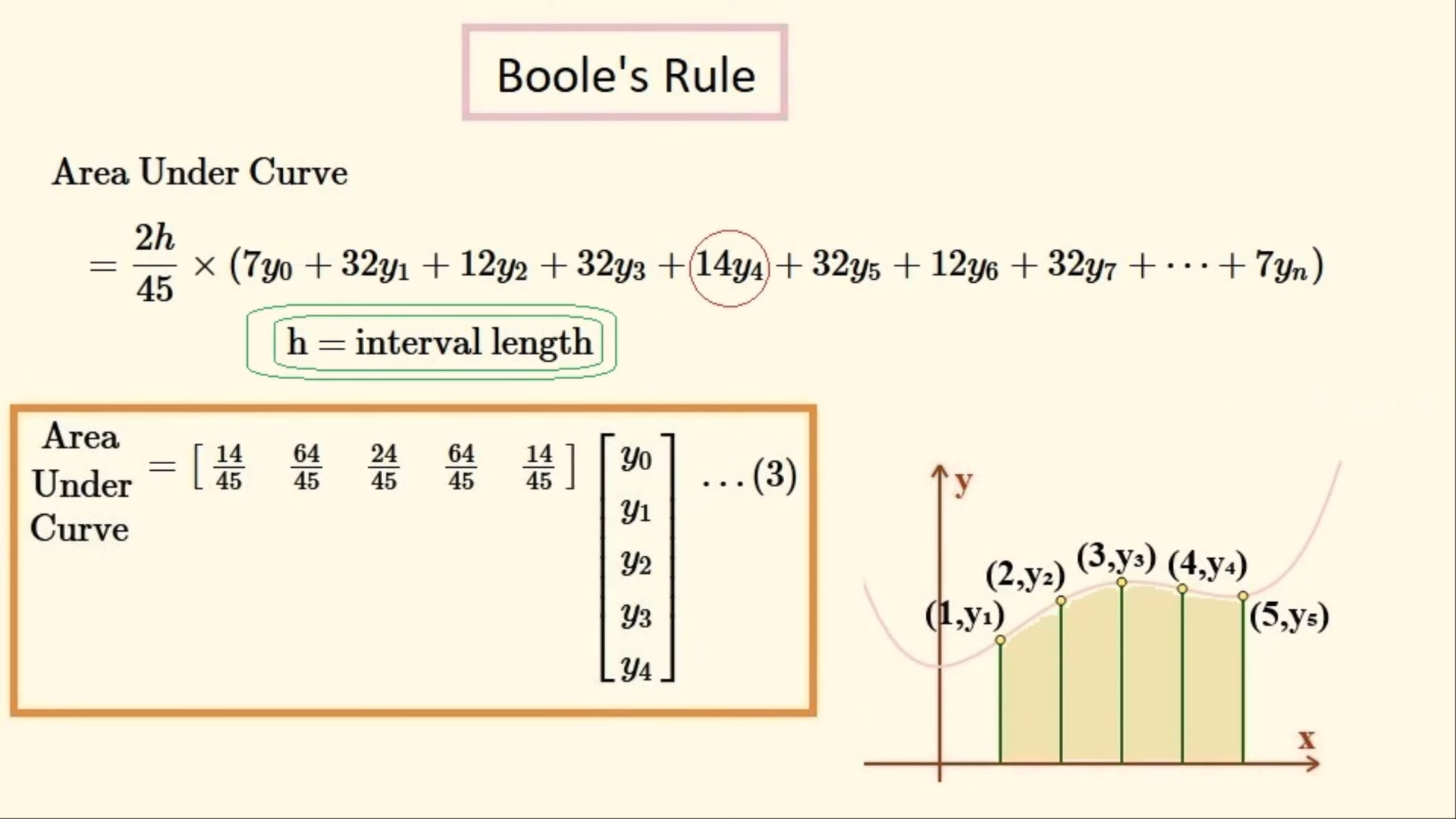
Boole's Rule

The Boole's rule is an improvement of the Simpson's rule with an even higher order of accuracy. It is 7th-order accurate, i.e. an error of order $O(h^7)$. Here, the composite Boole's rule will be used.

This rule approximates the integral via quartic interpolation, using a bunch of quartic functions that passes through five evenly spaced points in each subinterval. Such application of a higher-degree function in turn contributes to the enhanced accuracy of this method.

$$\int_{a}^{b}f(x)dx \approx {\frac {2h}{45}}\left(7(f(a)+f(b))+32\left(\sum _{i\in \{1,3,5,\ldots ,N-1\}}f(x_{i})\right)+12\left(\sum _{i\in \{2,6,10,\ldots ,N-2\}}f(x_{i})\right)+14\left(\sum _{i\in \{4,8,12,\ldots ,N-4\}}f(x_{i})\right)\right) \text{ where } h=\frac{b-a}{n}$$

An illustration of Boole's rule (screenshot taken from https://www.youtube.com/watch?v=CnDYKz3TeBo)

def integral_comp_boole(f, a, b, n):
    '''
    This function takes in the following parameters:-
    f: function to be integrated,
    a: lower limit of integration,
    b: upper limit of integration,
    n: number of subintervals in the partition of the integration interval, where n is divisible by 4,
    and outputs the value of the integral approximated using the composite Boole's rule.
    '''
    if n % 4 != 0:
        raise ValueError("n must be divisible by 4")
    h = (b - a)/n
    def term(i):
        t, c = a + i * h, None
        if i == 0 or i == n:
            c = 7
        elif i % 4 == 1 or i % 4 == 3:
            c = 32
        elif i % 4 == 2:
            c = 12
        elif i % 4 == 0:
            c = 14
        return c * f(t)
    return (2*h/45) * sum(term, 0, lambda i: i + 1, n) # sum function defined as above

cube = lambda x: x*x*x
print(integral_comp_boole(cube, 0, 1, 4)) # 0.25, exact value: 0.25 (set n = 4)

References, further reading

• Chang, X.-W. (2023). Numerical Integration. (McGill University COMP 350 Numerical Computing, Fall 2023 Teaching Slide)
• Pflueger, N. (2011). Math 1B, lecture 4: Error bounds for numerical methods.
• Composite Rules. Harvey Mudd College.

Footnotes

1. The trapezium rule, Simpson's rule and Boole's rule are part of a bigger family of numerical integration methods called Newton-Coles formulae. ↩

2. The fact that the sum function can be reused multiple times like this demonstrates the benefit of functional abstraction and higher-order functions in terms of code clarity. ↩